Deep learning statistical arbitrage part 1 - replication
Introduction
I first came across the paper Deep learning statistical arbitrage by Jorge Guijarro-Ordonez, Markus Pelger, and Greg Zanotti, back in 2022. I thought the strategy described in the paper was clear and intuitive, and it was the first time the concepts of statistical arbitrage really clicked for me. The headline results, a Sharpe ratio of ~4 in frictionless out-of-sample trading from 2002-2016, were impressive, and I wanted to test the ideas on my own data. The authors did provide a python repo, but it’s abandoned academic code.
Here, I reproduce the results of the paper with a clean, from-scratch pytorch implementation. I reach parity with the paper’s results in nearly all of the key sections, and I think the remaining shortcomings are mainly due to differences in data. I’m releasing the code to reproduce these results on your own data as well. Future posts will look at extending the time horizon to 2025, extensions to new stock universes, and other possible improvements to the model.
Background
Statistical arbitrage (stat arb) is a generalization of the basic pairs trading (mean reversion) principle: find two stocks that are correlated, wait until they diverge, then go long one and short the other until they converge again. Capturing the convergence of that spread is your profit. Stat arb extends pairs trading to a portfolio of hundreds or thousands of stocks to exploit pricing anomalies across the entire market. Using quantitative models, traders can construct market and factor-neutral portfolios that capture mean reversion of the entire group, rather than just the behavior of a single pair.
Methods
“Deep learning statistical arbitrage” builds portfolios that contain the most liquid ~550 stocks and trades once per day. The strategy has three key parts:
- Build the arbitrage portfolios. Every day, strip the common factors out of each stock’s return using one of three methods: regression on Fama-French factors, principal component analysis (PCA), or instrumented principal component analysis (IPCA). What remains are the residuals, the stock-specific features that the broad market doesn’t explain. Trading residuals instead of raw returns is what keeps the book market-neutral.
- Read a signal from each residual. Feed the last 30 days of a stock’s residual path into a small neural network. The paper’s headline results use a convolutional neural network (CNN) followed by a one-layer transformer. The network’s output is one number per stock.
- Turn the signals into a portfolio. While other stat arb methods might optimize the allocation function in a separate third step, here the network’s outputs are the portfolio weights. The CNN+Transformer is trained to maximize one thing: the Sharpe ratio of the resulting long/short book.
Data
I use daily US stock returns scraped from a few different sources, and daily factor and risk-free rate data from the Ken French data library. The authors trade large-cap stocks that have a market cap greater than 0.01% of the total market cap of the previous month, which equates to roughly 550 stocks. I had to set the threshold at 0.025% to give an average of 540 names.
The instrumented principal component analysis (IPCA) ties each stock’s factor loadings to its firm characteristics, and the paper’s strongest version leans on company fundamentals I didn’t initially have. I found Open Source Asset Pricing could get me most of the way there: pairing 32 of its fundamental signals with calculated price-based characteristics gives a total of 56 characteristics, close enough to the 46 the paper uses.
Model architecture and training
I matched the paper’s model architecture and training setup exactly: a rolling 1000-day window, retrained every 125 days, plain Adam, 100 epochs. The headline training objective is portfolio Sharpe, but I also ran the mean-variance version.
Results
The strategy mostly reproduces
For this post I follow the paper exactly: residuals built from 1998 onward, and out-of-sample testing from 2002 to 2016. The results reported here are annualized Sharpe ratio, mean returns, and volatility. α% is the return that the Fama-French 8-factor model can’t explain, and t(α) is that alpha’s t-statistic, where anything above 2 is statistically significant. A high alpha with a high t-statistic is the signature of a real edge, not just disguised exposure to known factors (beta, momentum, etc).
K is how many common factors the model removes before trading the leftover residual: the number of principal components for PCA, factors for Fama-French, or instrumented latent factors for IPCA.
| Factor / K | This replication | Paper | ||||||||
|---|---|---|---|---|---|---|---|---|---|---|
| Sharpe | μ % | σ % | α % | t(α) | Sharpe | μ % | σ % | α % | t(α) | |
| PCA K1 | 2.74 | 6.6 | 2.4 | 6.6 | 11.4 | 2.74 | 15.2 | 5.5 | 14.9 | 10.0 |
| PCA K3 | 3.13 | 6.7 | 2.1 | 6.6 | 9.8 | 3.56 | 16.0 | 4.5 | 15.8 | 14.0 |
| PCA K5 | 3.40 | 6.7 | 2.0 | 6.5 | 10.9 | 3.36 | 14.3 | 4.2 | 14.1 | 13.0 |
| PCA K8 | 3.37 | 6.2 | 1.8 | 6.0 | 10.4 | 3.02 | 12.2 | 4.0 | 12.0 | 12.0 |
| PCA K10 | 3.07 | 5.6 | 1.8 | 5.4 | 9.5 | 2.81 | 10.7 | 3.8 | 10.5 | 11.0 |
| PCA K15 | 2.82 | 5.1 | 1.8 | 4.9 | 8.7 | 2.30 | 7.6 | 3.3 | 7.5 | 8.8 |
| IPCA K1 | 3.25 | 8.1 | 2.5 | 7.6 | 12.8 | 3.22 | 8.7 | 2.7 | 8.1 | 12.0 |
| IPCA K3 | 3.99 | 8.3 | 2.1 | 7.9 | 13.0 | 3.93 | 8.6 | 2.2 | 8.2 | 15.0 |
| IPCA K5 | 3.98 | 7.7 | 1.9 | 7.4 | 11.5 | 4.16 | 8.7 | 2.1 | 8.3 | 16.0 |
| IPCA K8 | 3.81 | 7.1 | 1.9 | 7.0 | 12.2 | 3.95 | 8.2 | 2.1 | 7.8 | 15.0 |
| IPCA K10 | 3.74 | 7.0 | 1.9 | 6.8 | 12.3 | 3.97 | 8.0 | 2.0 | 7.7 | 15.0 |
| IPCA K15 | 3.57 | 6.8 | 1.9 | 6.6 | 11.7 | 4.17 | 8.4 | 2.0 | 8.1 | 16.0 |
| FF K1 | 2.89 | 7.1 | 2.4 | 6.8 | 10.8 | 3.68 | 7.2 | 2.0 | 7.0 | 14.0 |
| FF K3 | 2.74 | 6.3 | 2.3 | 6.1 | 9.4 | 3.13 | 5.5 | 1.8 | 5.5 | 12.0 |
| FF K5 | 2.30 | 4.9 | 2.1 | 4.6 | 7.4 | 3.21 | 4.6 | 1.4 | 4.5 | 12.0 |
| FF K8 | 1.92 | 4.0 | 2.1 | 3.8 | 5.5 | 2.49 | 3.4 | 1.4 | 3.3 | 9.4 |
For the all of the factor models, my implementation reproduces the Sharpe ratio trends of the paper:
- PCA: Max Sharpe of 3.40 at K=5 versus the paper’s 3.56 at K=3, with the same saturation as you remove more factors.
- IPCA: Nearly identical results at K=3, but the paper achieves higher Sharpe at higher K, while my results fade.
- Fama-French: Similar trends of highest Sharpe at low K, but I only achieve 80% of the paper’s top result.
One thing I’m still investigating is why my mean return in PCA is about half the paper’s. The Sharpe and t(α) are comparable, so the paper’s mean is achievable with leverage, but this discrepancy is one I haven’t been able to track down yet. It’s not a problem with IPCA.
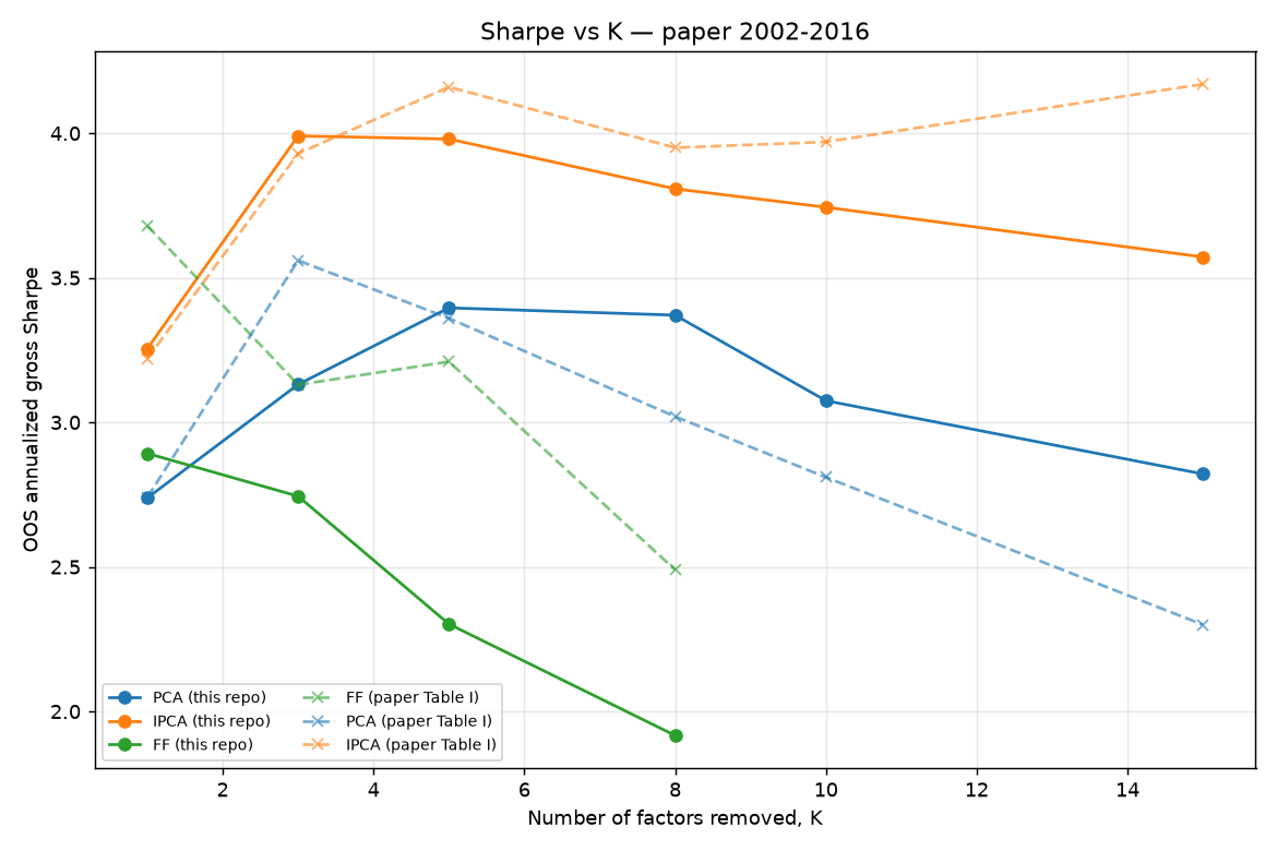 Out-of-sample Sharpe as more factors are removed for PCA, IPCA, and Fama-French portfolios, 2002-2016. Solid lines are mine, dashed are the paper’s.
The neural network is essential
The paper’s claims that the CNN+Transformer model beats a simpler network and classic mean reversion processes. That’s clearly true. The flexible signal the CNN+Transformer learns is responsible for multiples of Sharpe over the simpler models.
| Model (PCA K5) | This repo Sharpe | Paper Sharpe |
|---|---|---|
| CNN+Transformer | 3.40 | 3.36 |
| Fourier+FFN | 2.11 | 1.98 |
| Raw FFN (no signal extractor) | 1.10 | 1.42 |
| Classical OU + threshold | 1.16 | 0.73 |
Equity curves match the paper
I don’t think the authors distributed their return curves, so I can’t make an exact comparison here. I can say that the curves visually match what they present in Figure 5.
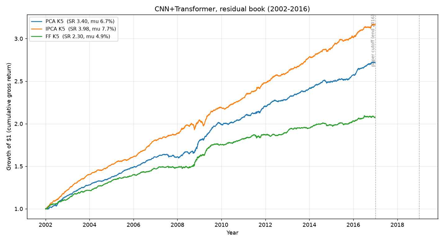 Growth of $1 for the CNN+Transformer book, 2002-2016. PCA and IPCA climb smoothly while the Fama-French book experiences greater volatility and drawdowns.
Portfolios you can actually trade: residual vs. stock-space returns
This paper, and most of the statistical arbitrage literature, shows returns of residual portfolios. That’s great for academics, but to actually trade this strategy, you don’t hold residuals, you hold stocks! We have to map the residual portfolio weights back to stock space through the Φ matrix, then re-normalize the portfolio to gross leverage of 1. The paper covers the math, I’ll just discuss the implications here.
For PCA and IPCA, the residual portfolios are portfolios of the universe’s traded stocks. Each factor K we remove is just a weighted basket of the same universe. Trading the PCA or IPCA portfolio is nearly identical to trading the residual portfolio.
The Fama-French portfolios are different. The FF factors are calculated from a much larger universe, so the residual portfolio is no longer expressible only in terms of stocks we’re capable of trading. When we map the residuals back to stocks in our universe, we lose some of the hedged factor exposure. The FF strategy ends up about 26% net long, picks up a 0.30 market beta, and its Sharpe falls from 2.30 to 0.97.
You can see it in the equity curves. As residuals (the figure above) all three portfolios climb smoothly. As tradable stock positions, PCA and IPCA are nearly unchanged, but Fama-French becomes choppy with real drawdowns.
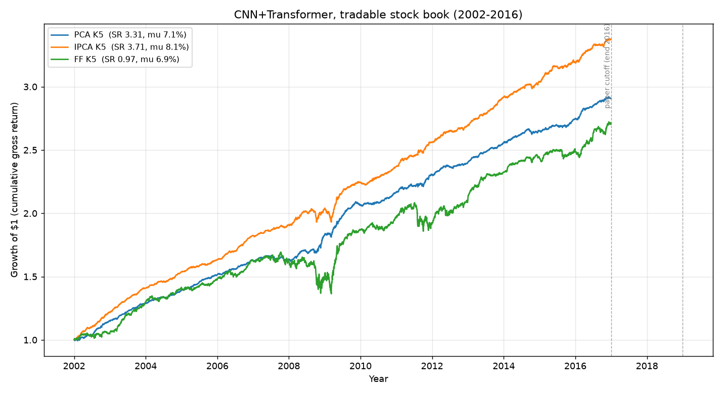 The same three books as tradable stock positions instead of pure residuals. PCA and IPCA are nearly unchanged from the residual version, while Fama-French picks up added volatility once it’s made tradable.
A second objective: mean-variance
Everything above maximizes the Sharpe ratio, which is the paper’s main objective. The paper also reports a mean-variance objective, which maximizes annualized mean minus annualized volatility, It’s supposed to trade a little risk-adjusted performance for a higher average return. I was able to replicate the key characteristics of this result as well. For example, PCA K=5 has a slightly lower Sharpe but higher returns, with the same leverage=1 constraint.
| Factor / K | This replication | Paper | ||||||||
|---|---|---|---|---|---|---|---|---|---|---|
| Sharpe | μ % | σ % | α % | t(α) | Sharpe | μ % | σ % | α % | t(α) | |
| PCA K1 | 2.56 | 13.4 | 5.3 | 13.3 | 7.9 | 2.21 | 27.3 | 12.3 | 26.3 | 8.3 |
| PCA K3 | 2.67 | 10.3 | 3.9 | 10.0 | 8.4 | 2.38 | 22.6 | 9.5 | 22.1 | 9.1 |
| PCA K5 | 2.97 | 10.3 | 3.5 | 9.8 | 9.4 | 2.75 | 19.6 | 7.1 | 19.0 | 10.0 |
| PCA K8 | 2.79 | 8.3 | 3.0 | 8.1 | 9.1 | 2.68 | 16.6 | 6.2 | 16.3 | 10.0 |
| PCA K10 | 2.71 | 7.2 | 2.6 | 6.9 | 9.1 | 2.67 | 15.3 | 5.7 | 14.8 | 10.0 |
| PCA K15 | 2.93 | 6.9 | 2.3 | 6.6 | 9.2 | 2.20 | 8.7 | 4.0 | 8.5 | 8.4 |
| IPCA K1 | 2.59 | 12.4 | 4.8 | 10.7 | 8.4 | 2.83 | 15.9 | 5.6 | 14.0 | 11.0 |
| IPCA K5 | 2.86 | 11.2 | 3.9 | 10.2 | 8.9 | 3.21 | 18.2 | 5.7 | 16.7 | 12.0 |
| IPCA K15 | 2.84 | 8.7 | 3.1 | 8.1 | 9.5 | 3.34 | 16.3 | 4.9 | 14.8 | 13.0 |
Conclusions
The major conclusions from “Deep learning statistical arbitrage” reproduce categorically. Without the exact data files from the authors, I can’t expect to exactly hit their numbers, so I’m satisfied with where I got to.
The CNN+transformer network is small and trains easily on a desktop GPU at the modest universe sizes we’re talking about here. This has been a fun model to learn statistical arbitrage with!
- PCA CNN+Transformer, the paper’s main model, reproduces cleanly.
- The model ranking holds: CNN+Transformer > shallow network > classic mean-reversion.
- The returns are real alpha, and significant in the 2002-2016 time period considered.
- IPCA, instrumented with OSAP fundamentals, reproduces at low K.
- The mean-variance objective behaves as advertised: lower Sharpe, higher average return.
Next up
There’s some obvious next steps after this work, such as extending the time horizon to a more recent date, expanding on the cost constraints and trading frictions, applying sparsity to the residuals and traded stocks, and expanding the traded universe. I’ll tackle those in a future post.
Reproduction repo
I’ll publish this code soon once I clean it up; it’s a little full of AI slop at the moment. Importantly, I want others to be able to reproduce it after plugging in a data source.